Data modeling
Data modeling
The BI Flow consists of
ETL
Data Modeling
Data Visualization
ETL is handled with Power Query, while Data Modeling is done with Power Pivot
Data modeling: Complex analyses between several tables connected by a common field
Relations and filters
Relationships between tables
Primary keys: Used to define the primary key of the table. Columns that have this profile cannot contain null values and cannot have duplicate values. That is, it must contain unique records
Foreign keys: A foreign key is a column or set of columns, which contains a value that refers to a row of another table
Relationship types:
1:1 (from 1 to 1): Both tables are connected by their primary keys. It acts as an extension of these
1:n (from 1 to several): Occurs when a primary key is connected with the foreign key of another table
m:n (many-to-many): Occurs when both tables are related by their foreign keys (none of the columns have unique values). Avoid these kinds of relationships
Conflicts to resolve:
Relationships m:n: By means of the concatenation of key fields or by means of associative tables
Inactive Relationships:
Delete them because they are not necessary
They can be unresolved relationships m:n
The Model Documenter tool is very interesting
Design of data models:
There are different types (star, snowflake, etc.)
In Power BI, we focus on the star schema model, which is the most efficient
Star model components:
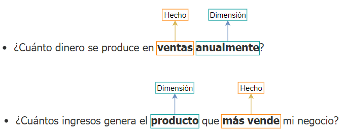
Fact tables: Also known as transactional tables or (fact in English). They answer the question of what do I want to obtain or look for?
Dimension tables: Also known as lookup tables. They respond to the level of classification that interests us, which can be time or type of data
Data model engine
His name is Vertipaq
Handles all data analysis operations (DAX)
Uses in-memory technology that provides high storage and performance in the data query
Allows short development cycles
Fixing modeling issues
Data Model Design: The Star Schema Model is the most used in Power Bi because it is made up of a dimension table (Search) and a Fact table (transactional) where the integration of both excels the one-to-many relationship and thus avoids data redundancy
Data Model Engine: VERTIPAQ is in charge of data analysis operations (DAX) and uses technology (in-memory) that provides high performance to store and query data
Need for data modeling:
If a single dashboard is loaded, it will have poor performance for large data volumes and with data redundancy
Proper modeling avoids these problems
DAX language
DAX (Data Analysis Expression):
Power BI Analytical Expression Language: Uses analytical formulas and operational functions that allow the calculation of one or more values
Created to manipulate a tabular data model
It is based on Excel; hence their similarity in terms of formulation structure. We can find this language in Power BI, SAS Tabular, and Excel in the Power Query plugin
Why DAX?:
Navigation Relations.
Designed to reach a greater number of users
Dynamic calculation of dimensions, for example, Time Intelligence
The shorter learning curve for data analysts. Leverage existing knowledge of working with Excel formulas
For example: = IF (Sales > 0, "WON", "LOST")
What can we create with DAX?
Calculated Columns: This allows methods to create new columns in the data model. It also allows tables with multiple key columns to be connected in a new column.
Calculated Tables: Creates a table derived from another table. For example, this system allows us to create tables without duplicates of a field from another table, to break relationships m:n
Measures: Supports time intelligence and creates dynamic calculations, which is the most used in Power BI
Language conventions (general format):
'table name' [column name]. Example: 'Products table'[Price]
The table name can be omitted when used in calculated columns, but it is not recommended to do so.
Use CALCULATE
'table name' [column name]. Example: 'Products table'[Price]
The table name can be omitted when used in calculated columns, but it is not recommended to do so
Time intelligence
By time Intelligence, we refer to the techniques, tools, and methodologies that allow us to analyze our measurements carefully over time
The concept of "time" is present in all business intelligence solutions. It serves as a starting point to exploit the information
Table of dates
In order to use this type of analysis within Power BI, we will first need to create a new dimension
These tables are known as date tables or calendar tables, and they function as a new dimension for our model.
A table of dates is identified by having all the dates existing in our model (or at least those necessary for the analysis) continuously. That is, without missing a single day between the dates
Allows you to monitor growth or decline in detail
Allows projections
Iterators X
Iterative functions
These types of functions are special within DAX and allow you to create operations at the row level and calculate a result from them
Iterative functions are also known as X functions, because of their ending within their name in DAX
Some of these functions are: SUMX, AVERAGEX, MAXX, MINX, STDEVX.S, PERCENTILEX.EXC and CONCATENATEX
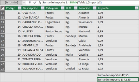
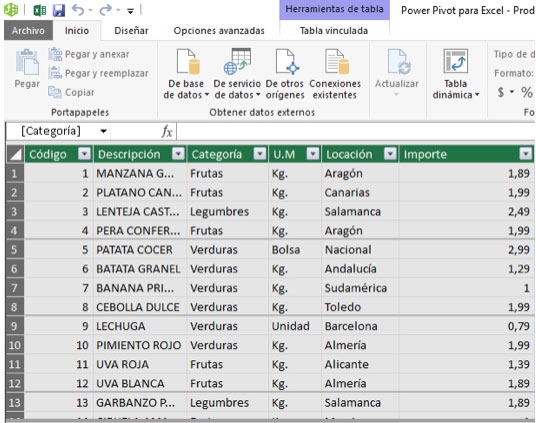
SUM and SUMX simulations in Excel:
We need to calculate the sum of the amount of all the products. What function should we use? Can we use one or the other interchangeably?
SUM:
Add all the numbers in a column.
The parameter is the column that contains the numbers to add. The function accepts numeric or date values and returns a decimal value as a result. Rows can contain blank values. Column values cannot be filtered.
Sum of Amount := SUM([Amount])
SUMX:
Returns the sum of an expression evaluated for each row of a table
The parameter is the table containing the values for which the expression will be evaluated. Can be the name of a table or an expression that returns a table. The parameter is a column that contains the numbers you want to sum, or an expression that evaluates to a column. Only the numbers in the column are counted. White space, logical values, and text are ignored.
Sum of Amount 1 := SUMX(Table1; [Amount])
We can see that the two functions return the same result. What differentiates both functions is the way they perform the calculation: The SUMX function is an iterator, it will go through each row evaluating an expression while the SUM() function will directly add the column values. For this case the SUM() function is recommended
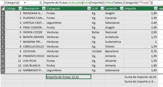
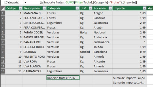
2. Calculate the sum of the Amount of the previous model only for the white fruit category
SUM:
The SUM() function does not allow us to filter the rows of the table on which we want to perform the calculation, and we must combine it with the CALCULATE() function. Fruit amount := CALCULATE(SUM([Amount]) ; Filter(Table1;[Category]=”fruit”))
SUMX:
On the other hand, the SUMX () function does allow us to: Import fruits := SUMX(Filter(Table1; [Category]=”fruit”); [Amount])
In this case, either of the two could be used, if applied in an aforementioned manner
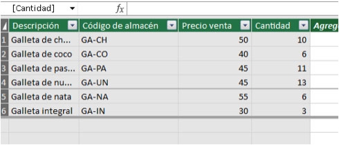
3. Calculate total sales. In this model, unlike the previous one, we do not have a column with the amount of each row, but we can calculate it using the Sale Price and Quantity columns in the expression:[Sale Price]*[Quantity]
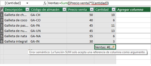
SUM:
Syntax: SUM([Sale Price]*[Quantity])
The SUM() function returns an error because it only accepts one column as a parameter
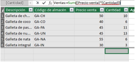
SUMX:
On the other hand, the SUMX() function does allow us to do this because it supports an expression in addition to a column:
Syntax: SUMX(Table2;[Sale Price]*[Quantity])
In this case the SUMX() function is recommended
Last updated